Google's AutoML has attracted a lot of attention from the academic community and the industry. However, behind its simple operation, it is a large amount of scientific research supported by powerful computing power. One of them is the progressive network structure search technology. In this article, Dr. Liu Chenxi will unveil the AutoML veil for everyone, and see how he can find the optimal network structure through iterative self-learning, and find the best network structure.
At the end of the article, the lecture hall specifically provides download links for all articles and codes mentioned in the article.
In this paper, the progressive neural network search algorithm introduced will be completed together with many researchers at Google Brain, Google Cloud, and Google Research Institute.
Among them, the code and model of PNASNet-5 on ImageNet has been released in TensorFlow Slim:

First, introduce AutoML, which is an ambitious goal within Google. It is to create a machine learning algorithm that best serves the data provided by the user, with as little human involvement as possible.
From the initial AlexNet to Inception, ResNet, Inception-ResNet, the machine has achieved good results in image classification, so why do we want to use AutoML algorithm to study image classification?
First of all, if you can find an algorithm that is better than the best algorithm designed by humans through automatic search, isn't it cool? Secondly, from a more practical point of view, the problem of image classification is a problem that everyone learns a lot. If a breakthrough is made on this issue, the possibility of breaking through other problems is greatly increased.
Next, we will introduce the Neural Architecture Search (NAS) problem, which is a specific branch of AutoML.
Neural Architecture Search basically follows a cycle: first, create a simple network based on some policy rules, then train it and test it on some verification sets, and finally optimize these policy rules based on feedback of network performance, based on these optimized The strategy is to iteratively update the network.
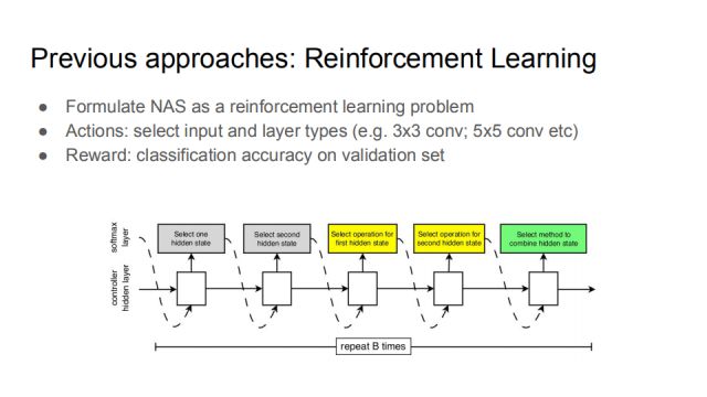
The previous NAS work can be roughly divided into two aspects. The first is reinforcement learning. In the neural structure search, many elements need to be selected, such as input layer and layer parameters (such as convolution operation with 3 or 5 core selection). The process of the entire neural network can be seen as a series of actions, and the reward of the action is the classification accuracy rate on the verification set. By constantly updating the actions, the agent learns a better and better network structure, so that reinforcement learning and NAS are connected.
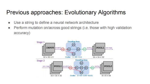
On the other hand, NAS is an evolutionary algorithm. The main idea of ​​this large class of methods is to define a neural network structure with a series of numbers. The picture shows the work of Dr. Xie Lingwei of ICCV2017. He uses a string of binary codes to define a rule to express a specific neural network connection. The initial code is random. From these points, you can make some mutations, even in two numbers. Mutations between strings (with high verification accuracy) can provide a better neural network structure over time.
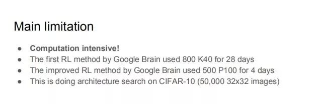
The biggest problem with the current method is that it has a particularly high demand for computing power. Taking reinforcement learning as an example, Google’s brain first proposed an intensive learning method that used 800 K40 GPUs and trained for 28 days. Later, the improved version proposed in July 2017 was trained with 500 P100 GPUs for 4 days, and this is Made on a very small CIFAR-10 dataset, the dataset has only 50,000 30*30 maps. Even such a small data set needs such a large amount of computing power, that is to say, if you want to continue to expand the NAS, it is unrealistic to use the method of reinforcement learning.

To speed up the NAS process, we propose a new method called "progressive neural structure search." It is neither based on reinforcement learning nor an evolutionary algorithm. Before introducing a specific algorithm, first understand the search space here.
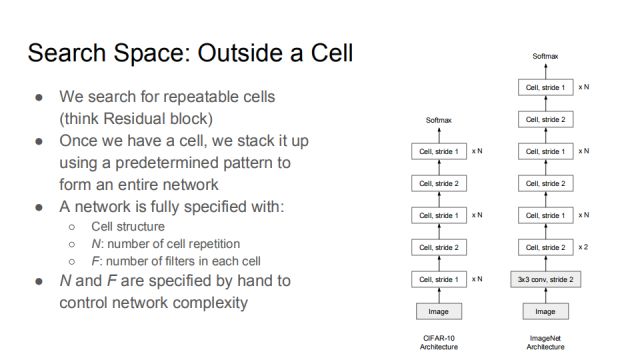
First search for repeatable cells (can be regarded as Residual block), once you find a cell, you can freely choose the stacking method to form a complete network. Such a strategy has appeared multiple times in the Residual Network. After the cell structure is determined, it is superimposed into a complete network as shown in the right figure. Taking the CIFAR-10 network as an example, between the cells of the two stride2, the number of cell superpositions of stride1 is N, and different groups in the Residual network. The number of overlays is different.
A network is usually determined by these three elements: the structure of the cell, the number of times the cell is repeated N, and the number of convolution kernels F in each cell. In order to control the complexity of the network, N and F are usually designed by hand. It can be understood that N controls the depth of the network, and F controls the width of the network.
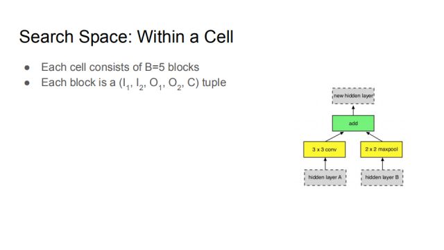
Next, we mainly discuss how to determine the cell. In our search space, a cell consists of 5 blocks, and each block is a tuple of (I_1, I_2, O_1, O_2, C). The details will be described below.
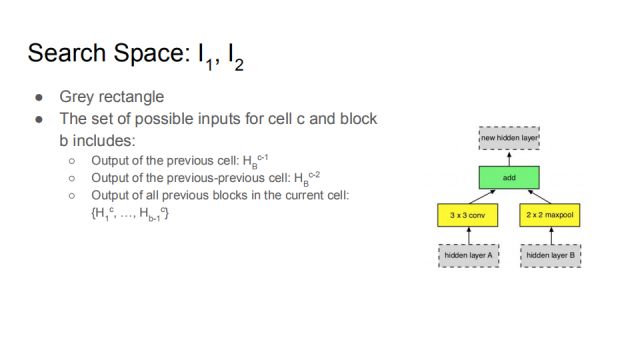
As shown in the figure, the search space of the network input is shown by the gray rectangle in the figure, I_1, I_2 corresponds to the hidden layer A and the hidden layer B, and I refers to the input (Input). The two gray blocks can choose different implicit spaces. The possible input of cell c block b is defined as:
Output of the previous cell: H_B^(c-1)
The output of the previous previous cell: H_B^(c-2)
Output before all current blocks of the current cell: {H_1^c,...,H_(b-1)^c }
For example, the block on the right is the first block in the cell. When the second block is selected, it can select the new hidden layer generated by the first block. That is, the input of the second block covers the first block. The output of the block. Such a design can portray networks such as Residual Network and DenseNet in order to allow for certain generalization.
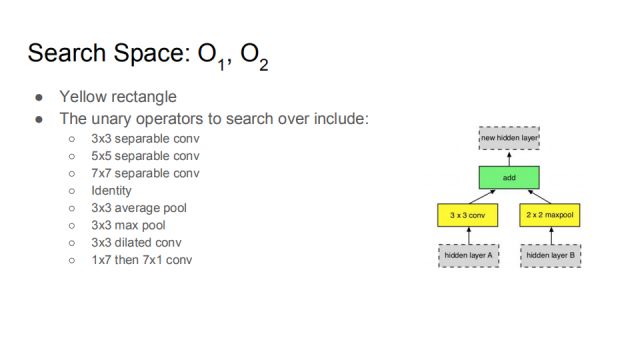
O_1, O_2 corresponds to the yellow box in the figure. This is actually the unary operator of the hidden layer just selected. It contains a 3*3 convolution, a 5*5 convolution, and a 7*7 convolution. Identity, 3*3 mean pooling, 3*3 maximum pooling, 3*3 widening pooling, and 1*7 followed by 7*1 convolution. Let the data learn in the search space to find the most suitable operation.
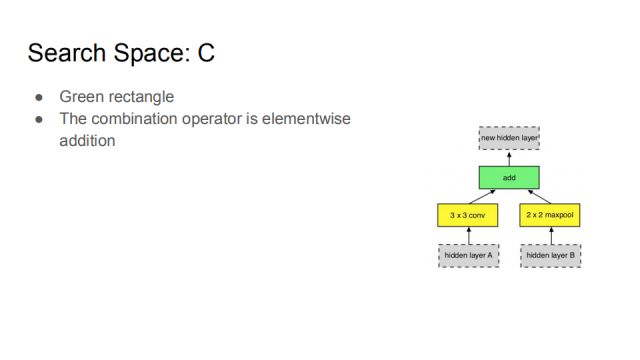
The green box represents the C operation, which combines O_1 and O_2 generated by I_1, I_2 in a certain way to create a new implicit space. This C operation is a bitwise sum operation.
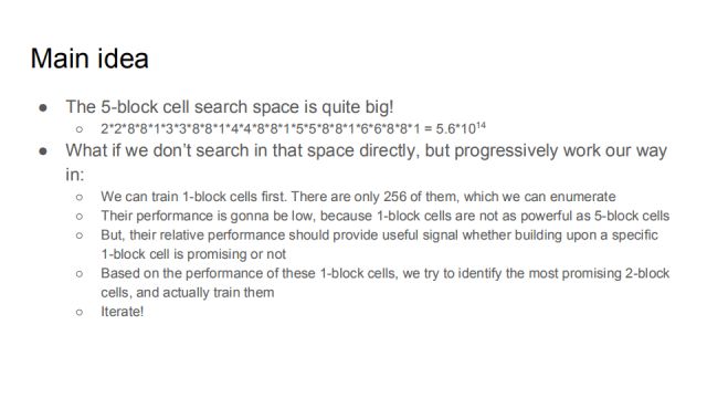
In this search space, learn a cell with better performance as effectively as possible, so that it can be superimposed into a complete network. The search space of the cell containing just 5 blocks is very large, as shown in the above equation. The previous introductions, whether reinforcement learning or evolutionary algorithms, are direct searches, which is very confusing at the beginning of the search, so what if you do not search directly in that space, but proceed progressively as follows:
First train all 1-block cells, only 256 such cells. Although it can be enumerated, the performance will be low, because only one block of cells is not as efficient as a cell containing 5 blocks. However, this part of the performance information can provide assistance for whether to continue to use the signal of this cell. Based on the performance of 1-block cell, we can try to find the most promising 2-block cell and train it. Build the entire network.
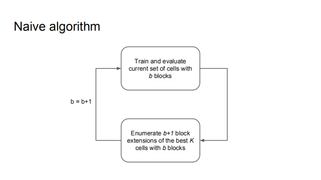
It can be summarized as a simple algorithm that trains and evaluates cells that currently have b blocks, then enumerates b+1 blocks based on the best K cells, and then trains and evaluates.
In fact, this algorithm can't really work, because, for a reasonable K (such as [10]^2), the sub-network that needs to be trained is as high as 〖10〗^5, and this calculation has exceeded the previous one. method. Therefore, we propose an accuracy rate predictor that can evaluate whether a model has potential without observing and testing, but by observing the number of strings.

We used an LSTM network to make an accuracy predictor, which was used because the same predictor could be used in different blocks.
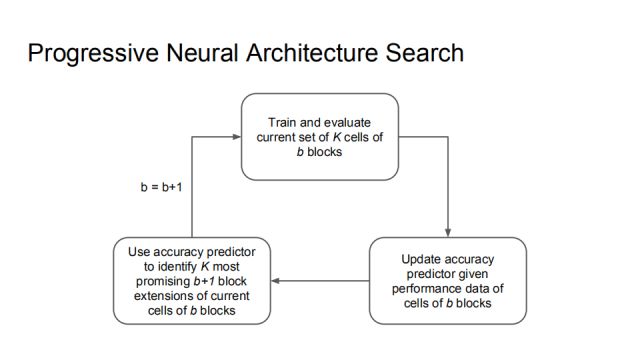
Here is the complete algorithm for Progressive Neural Architecture Search. First, train and evaluate the K cells of the current b blocks, and then update the accuracy predictor by the performance of these data, which can make the accuracy predictor more accurate, and use the predictor to identify the K most likely b+1 blocks. . The result of this learning may not be the most correct, but it is a reasonable trade-off result.

For example, at the beginning b=1, there are 256 networks in Q1, all of them are trained and tested, and then the K data points are used to train the accuracy predictor. All the descendants M1 of Q1 are enumerated, and this accuracy predictor is applied to each element of M1, and the best K is selected, that is, the set Q2 when b=2 is obtained. Then the network with b=2 is trained and tested. After the same process as above, Q3 can be obtained. The best model in Q3 is the result returned by PNAS.
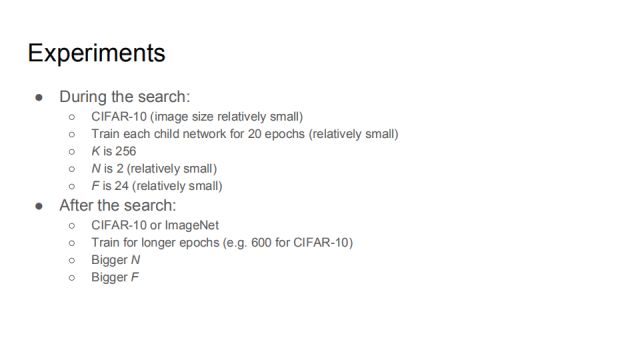
The experiment is divided into two processes, one in the search process and the other after the search. In the search process, we use CIFAR-10, a relatively small data set. The epoch of each subnet training is set to 20, K is 256, N is 2, and F is 24. These parameters are relatively small. of. After the search, we tested on CIFAR-10 and ImageNet, using longer epochs, larger N, F. The purpose of our work is to accelerate the process of NAS. The following is an experimental comparison.

Next, compare PNAS with the previous NAS method, the blue point is PNAS, the red one is NAS, and the five blue chunks correspond to b=1, 2, 3, 4. There are 256 points in each chunk, and as b increases, it moves into more and more complex search spaces. It can be seen that the blue point rises faster and more tightly than the red point. On the right is an enlarged view.
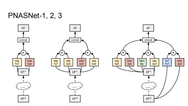
As shown in the figure, the network structure that was last learned can be seen that the combination of separable and max convolution was first learned, and more combinations were gradually learned.
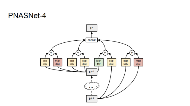
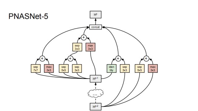
PNASNet-5 is the best network structure we found during the search process. It consists of 5 blocks.
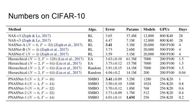
This is our comparison result on CIFAR-10. RL indicates that the algorithm is based on reinforcement learning, EA indicates that based on genetic algorithm, our algorithm SMBO is sequential model based optimization, and Error refers to the top-1 misclassification rate of the best model. The best of the first set of reinforcement learning based methods is NASNet-A, which has an error rate of 3.41% and the number of parameters used is 3.3M. The second group is based on the genetic algorithm method, which is DeepMind ICLR in 2018. Published work, its best error rate is 3.63%, the number of parameters used is 61.3M, and the third group is our method, under the condition of error rate of 3.41, we use only 3.2M, and speed up a lot of.
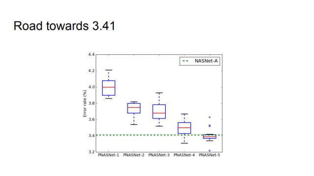
This picture shows more intuitively how to achieve comparable performance with NASNet-A.
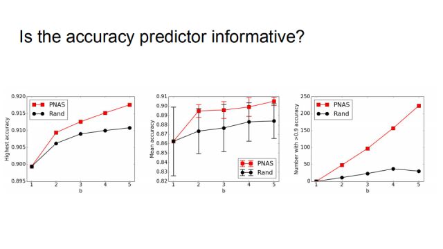
In order to verify that the accuracy predictor is informative, we did a random comparison experiment. If you do not use progressive neural architecture search, use random instead for each number of b. The results show that the performance of the random strategy is much worse, especially the far right. If 256 models are trained in each b value, the accuracy rate is greater than 0.9 as the statistical index, and the random method is only more than 30, while PNAS There are more than two hundred matches.
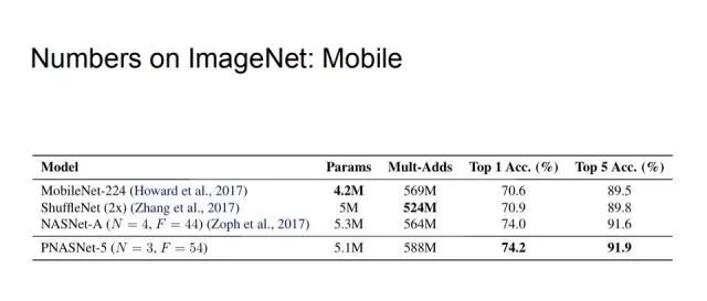
Finally, the comparison on the ImageNet dataset begins with an application comparison in lightweight neural networks. We control Mult-Adds to no more than 600M. Under this condition, PNASNet-5 has the highest top1 and top5 accuracy compared to MobileNet-224, ShuffleNet(2x), and NASNet-A.

In addition, the unconstrained models were compared, and the parameters of NASNet-A were kept as consistent as possible during the experiment, and the final top1 accuracy rate reached 82.9%.
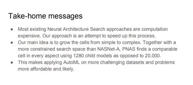
To sum up, the most critical points in the work presented in this report: Most existing neural network search methods have high computational demands, resulting in high time costs, and we are trying to speed up the process. The core of the idea is to push the cells from simple to complex, and with a tighter search space than NASNet-A, PNAS found a comparable cell, using only 1280 instead of 20,000 submodels. This allows AutoML to be used on more challenging data sets.
Alarm Accessories,Alarm Products,Alarm Equipment
Chinasky Electronics Co., Ltd. , https://www.cctv-products.com