1) Data collected
2) The hypothetical model, a function, which contains unknown parameters, can be estimated by learning. Then use this model to predict/classify new data.
Linear regressionAssume that the features and results are linear. That is no more than one time. This is for the collected data.
Each component of the collected data can be regarded as a feature data. Each feature corresponds to at least one unknown parameter. This forms a linear model function, vector representation:
![]()
This is a combination problem, some data is known, how to find the unknown parameters inside, and give an optimal solution. A linear matrix equation, solved directly, may not be directly solved. The data set with a unique solution is minimal.
Basically, it is a set of overdetermined equations that do not exist. Therefore, it is necessary to take a step back and transform the parameter solving problem into the minimum error problem and find a closest solution. This is a relaxation solution.
Find the closest solution, intuitively, you can think of the expression with the least error. It is still a linear model with unknown parameters, a pile of observation data, the smallest form of error between the model and the data, and the sum of the squares of the model and the data difference is the smallest:
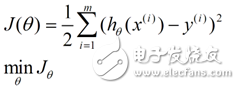
This is the source of the loss function. Next, there is a method for solving this function, which has a least squares method and a gradient descent method.
Least squares
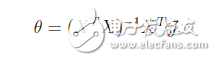
Is a straightforward mathematical solution, but it requires X to be full rank,
Gradient descent
There are gradient descent method, batch gradient descent method, and incremental gradient descent. Essentially, they are all partial derivatives, step size/best learning rate, update, and convergence. This algorithm is just an ordinary method in the optimization principle. It can be easily understood by combining the optimization principle.
2. Logistic regressionThe connection, similarities and differences between logistic regression and linear regression?
The model of logistic regression is a nonlinear model, sigmoid function, also known as logistic regression function. But it is essentially a linear regression model, because the sigmoid mapping function relationship is removed, and the other steps, the algorithm are linear regression. It can be said that logistic regression is supported by linear regression.
However, the linear model cannot achieve the nonlinear form of sigmoid, and sigmoid can easily handle the 0/1 classification problem.
In addition, its derivation meaning: still the same as the maximum likelihood estimation derivation of linear regression, the continuous product of the maximum likelihood function (the distribution here, can make Bernoulli distribution, or Poisson distribution and other distribution forms), derivation, Loss function.
![\begin{align}J(heta) = -\frac{1}{m} \left[ \sum_{i=1}^my^{(i)} \log h_heta(x^{(i)}) + (1-y^{(i)}) \log (1-h_heta(x^{(i)})) ight]\end{align}](http://i.bosscdn.com/blog/11/44/31/O12-3.png)
Logical regression function
It shows the form of the 0,1 classification.
Application examples:
Is spam classified?
Is it a tumor or cancer diagnosis?
Is it financial fraud?
3. General linear regressionLinear regression is a Gaussian distribution error analysis model; Logistic regression uses Bernoulli distribution analysis error.
Gaussian distribution, Bernoulli distribution, beta distribution, and Dietlet distribution all belong to the exponential distribution.
![]()
In general linear regression, under the condition of x, the probability distribution p(y|x) of y refers to the exponential distribution.
After deriving the maximum likelihood estimate, the error analysis model of the general linear regression (minimized error model) can be derived.
Softmax regression is an example of general linear regression.
There is supervised learning regression, for multiple types of problems (logical regression, solving the problem of two types of division), such as the classification of numerical characters, 0-9, 10 numbers, y value has 10 possibilities.
And this possible distribution is an exponential distribution. And if all possible sums are 1, then for an input result, the result can be expressed as:
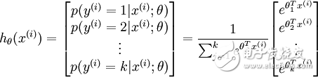
The argument is a k-dimensional vector.
And the cost function:
![\begin{align}J(heta) = - \frac{1}{m} \left[ \sum_{i=1}^{m} \sum_{j=1}^{k} 1\left\{y ^{(i)} = jight\} \log \frac{e^{heta_j^T x^{(i)}}}{\sum_{l=1}^ke^{ heta_l^T x^{(i )}}}ight]\end{align}](http://i.bosscdn.com/blog/11/44/31/2P5-7.png)
It is a generalization of the logistic regression cost function.
For the solution of softmax, there is no closed solution (high-order polynomial solution), and it is still solved by gradient descent method or L-BFGS.
When k=2, softmax degenerates into logistic regression, which also reflects that softmax regression is a generalization of logistic regression.
Linear regression, logistic regression, softmax regression, the three links, need to repeat the aftertaste, think more, understanding can go deeper.
4. Fitting: Fitting the model/functionFrom the measured data, an assumed model/function is estimated. How to fit, is the fitted model appropriate? Can be divided into the following three categories
Suitable fit
Under-fitting
Overfitting
I have read the illustration of an article (appendix) and it is very good to understand:
Under-fitting:
Appropriate fit
Overfitting
How to solve the problem of overfitting?
The origin of the problem? The model is too complex, with too many parameters and too many features.
Method: 1) Reduce the number of features, manually select, or use a model selection algorithm
2) Regularization, which preserves all features, but reduces the effect of the value of the parameter. The advantage of regularization is that each feature has a suitable impact factor when there are many features.
5. Probability interpretation: Why is square summation used as an error function in linear regression?
Assume that the model result and the measured value error are satisfied, and the Gaussian distribution with a mean of 0 is the normal distribution. This assumption is reliable and conforms to the general objective statistical law.
Conditional probability of data x and y:
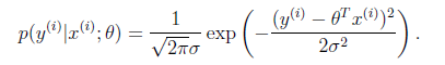
If the model is closest to the measured data, then the probability product is the largest. The probability product is the continuous product of the probability density function, thus forming a maximum likelihood function estimate. Deriving the maximum likelihood function estimate, the result after derivation is obtained: the sum of squares and the minimum formula
6. Parameter estimation and data relationship
Fitting relationship
7. Error function / cost function / loss function:
In the linear regression, the form of the sum of squares is generally derived from the maximum likelihood product of the conditional probability of the model, derived and derived.
In statistics, the loss function generally has the following types:
1) 0-1 loss function
L(Y,f(X))={1,0,Y≠f(X)Y=f(X)
2) Square loss function
L(Y,f(X))=(Y−f(X))2
3) Absolute loss function
L(Y,f(X))=|Y−f(X)|
4) Logarithmic loss function
L(Y,P(Y|X))=−logP(Y|X)
The smaller the loss function, the better the model, and the loss function is as much as possible a convex function, which is convenient for convergence calculation.
Linear regression uses a squared loss function. Logistic regression uses a logarithmic loss function. These are just some of the results, not deduced.
8. Regularization:
To prevent over-fitting models from appearing (overly complex models), add a penalty factor for each feature to the loss function. This is regularization. The loss function of linear regression such as regularization:
The lambda is the penalty factor.
Regularization is a typical method of model processing. It is also the least risky strategy. Add a penalty/regularization term based on the empirical risk (the sum of squared errors).
The solution of linear regression, also from
θ=(XTX)−1XTy
Converted to
The matrix in parentheses is reversible even if the number of samples is less than the number of features.
Regularization of Logistic Regression:
From Bayesian estimation, the regularization term corresponds to the prior probability of the model, the complex model has a large prior probability, and the simple model has a small prior probability. There are several concepts in this.
What is structural risk minimization? Priori probability? Is the relationship between the model simple and the prior probability?
Empirical risk, expected risk, loss of experience, structural risk
Expected risk (real risk) can be understood as the degree of loss of data average when the model function is fixed, or the degree of "average" error. The expected risk is dependent on the loss function and the probability distribution.
Only the sample is unable to calculate the expected risk.
Therefore, using empirical risk, estimate the expected risk and design the learning algorithm to minimize it. That is, Empirical Risk MinimizaTIon ERM, and empirical risk is calculated and calculated using the loss function.
For classification problems, empirical risk, the training sample error rate.
For function approximations, fitting problems, empirical risks, square training errors.
For the probability density estimation problem, ERM is the maximum likelihood estimation method.
The least risk is not necessarily the minimum risk and no theoretical basis. When the sample is infinite, the empirical risk approaches the expected risk.
how to solve this problem? Statistical learning theory SLT, support vector machine SVM is specifically to solve this problem.
Under a finite sample condition, learn a better model.
Due to the limited sample, the empirical risk Remp[f] cannot approximate the expected risk R[f]. Therefore, the statistical learning theory gives the relationship between the two: R[f] "= ( Remp[f] + e )
The expression on the right end is the structural risk, which is the upper bound of the expected risk. And e = g(h/n) is a confidence interval, which is an increasing function of the VC dimension h and a decreasing function of the number of samples n.
The definition of VC dimension is described in detail in SVM and SLT. e depends on h and n, if you minimize the expected risk, you only need to care about the minimum upper bound, that is, e minimized. Therefore, you need to choose the appropriate h and n. This is the structural risk minimization of Structure Risk MinimizaTIon, SRM.
SVM is an approximate implementation of SRM, and the concept in SVM has a big basket. Stop here.
1 norm, the physical meaning of 2 norm:
A norm that maps a thing to a non-negative real number and satisfies non-negative, homogeneous, and triangular inequalities. Is a function with the concept of "length".
Why can the 1 norm get a sparse solution?
Compressed sensing theory, solving and reconstruction, solving a least squares problem of L1 norm regularization. The solution is the solution of the underdetermined linear system.
Why can the 2 norm get the maximum interval solution?
The 2 norm represents the unit of measure of energy used to reconstruct the error.
The above concepts need to be understood.
9. Minimum description length criteria:
That is, a set of instance data, when stored, utilizes a model, encoding compression. The length of the model, plus the length after compression, is the total length of the description of the data. The minimum description length criterion is to select the model with the smallest total description length.
An important feature of the minimum description length MDL criterion is to avoid overfitting.
For example, using Bayesian networks to compress data, on the one hand, the length of the model's own description increases with the complexity of the model; on the other hand, the length of the description of the data set decreases as the complexity of the model increases. Therefore, the MD L of Bayesian networks always seeks to strike a balance between model accuracy and model complexity. When the model is too complex, the minimum description length criterion will work and limit the complexity.
Occam razor principle:
If you have two principles that explain the observed facts, then you should use the simple one until you find more evidence.
Everything should be as simple as possible, not simpler.
11. Convex relaxation technique:
Transform the combinatorial optimization problem into a convex optimization technique that is easy to solve extreme points. Derivation of convex/cost function, maximum likelihood estimation.
12. Newton method for solving maximum likelihood estimation
Precondition: Derivation iteration, likelihood function can be guided, and second order can be guided.
Iteration formula:
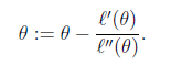
If it is a vector form,
![]()
H is the hessian matrix of n*n.
Characteristics: Newton's method can converge quickly when it is close to the extreme point, and Newton's method may not converge away from the extreme point. The derivation of this?
This is the opposite of the convergence characteristic of the gradient descent method.
Linearity and nonlinearity:
Linear, linear function; nonlinear, input and output are not proportional, non-primary functions.
Linear limitations: xor problem. Linear is inseparable, form:
x 0
0 x
Linear is separable, which uses only one linear function to classify the data. Linear function, straight line.
Linearly independent: individual features, independent components, cannot be represented linearly by other components or features.
The physical meaning of the kernel function:
Map to high dimensions to make them linearly separable. What is high dimensional? For example, a one-dimensional data feature x, converted to (x, x^2, x^3), becomes a three-dimensional feature and is linearly independent. A linearly indivisible feature of a one-dimensional feature may be linearly separable in high dimensions.
Logistic regression logicalisTIc regression is still linear regression in nature, why is it listed as a separate category?
There is a non-linear mapping relationship, and the processing is generally a 0,1 problem of the binary structure. It is an extension of linear regression and is widely used and is listed as a separate class.
And if you apply linear regression directly to fit the logistic regression data, many local minima are formed. It is a non-convex set, and the linear regression loss function is a convex function, that is, the minimum extreme point, that is, the global minimum point. The model does not match.
If the loss function of logistic regression is used, the loss function can form a convex function.
Polynomial spline function fitting
Polynomial fitting, the model is a polynomial form; the spline function, the model is not only continuous, but at the boundary, the high-order derivatives are also continuous. Benefit: It is a smooth curve that avoids the appearance of turbulence in the boundary (Longge linear)
Here are a few concepts that need to be understood in depth:
Unstructured predictive model
Structured prediction model
What is a structured problem?
Adaboost, svm, lr The relationship between the three algorithms.
The distribution of the three algorithms corresponds to exponenTIal loss, hinge loss, log loss, and no essential difference. The convex upper bound is used to replace the 0, 1 loss, that is, the convex relaxation technique. From combinatorial optimization to convex set optimization problems. Convex functions are easier to calculate extreme points.
Exhaust Fuel Pressure Sensor,Pressure Transducer,Water Pressure Sensor,Waterproof Pressure Sensor
Shenzhen Ever-smart Sensor Technology Co., LTD , https://www.fluhandy.com