Foreword
This article refers to the address: http://
Gps (Global Positioning System) is supported by 24 satellites and has global, all-weather, continuous navigation and positioning. Due to its high precision, high speed, low cost and convenient use, it has not only gained widespread attention in the military, but also has been applied more and more in the civil sector.
At present, domestic applications of GPS mainly focus on vehicle information service systems and railway and highway construction surveys. The survey of iron and highway routes can be divided into two situations. First, the need to construct routes, using GPS to locate the initial surveyed conductor points and benchmarks. First, collect route data from existing routes through GPS to restore the actual route map. . In the latter case, due to the factors of route collection point density and measurement error, in practical applications, it is necessary to use the obtained data to perform a certain fitting.
2 Background of the project
In China, the existing locomotive headlights are fixed. When the locomotive enters the corner, the light cannot be illuminated on the front rail in real time. Design an activity headlight, based on the locomotive route data, obtain the current position of the locomotive through GPS, and adjust the headlight corner in real time, which can greatly improve the safety of locomotive driving. The system block diagram is as follows:
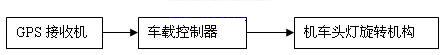
Figure 1 Block diagram of the locomotive headlight control system
In the on-board controller, the position and speed data obtained by the GPS receiver are compared with the pre-stored route data table, and finally the control corner signal quantity that needs to be sent by the current position of the locomotive is obtained. The pre-stored route data table needs to be processed in advance in the personal computer, the fit mentioned in the introduction. Whether in vehicle information service systems or other applications related to geographic routes, the collection and fitting of route data is an extremely important part.
3 GPS data collection
The data received by the GPS receiver is output in a serial port manner according to the data stream in a certain message format. Its format is:
$GP RMC,081546,A,105.7038,N,30.3624,E,0.000,0.0,220406,1.1,W*78
With a comma as a separator, each data item sequentially indicates the start mark of the new data frame, Greenwich Mean Time, data valid flag, latitude, north-south latitude mark, precision, east-west mark, moving speed, date, magnetic change, east-west magnetic Change the sign and checksum. For the fitting of the route, what is actually needed is the latitude and longitude of each point. For this reason, the extraction processing is required, which can be collected by the portable computer, and the communication between the computer and the GPS receiver is through the serial port, and the communication control can utilize the Microsoft company's The MSCcomm serial communication control is simple and flexible to program, and it can also directly call Windows API functions or dynamic link libraries for a richer design. There are many articles in these methods for special discussion. This article gives a brief introduction to the PC104 micro-board used in the system through serial communication. The PC104 micro-board is small in size, and the GPS receiver is still very compact and easy to carry. When the route data is collected, it is placed on the locomotive. The collected data is stored in its own FLASH. After the acquisition, it can be copied to the personal computer hard disk through the IDE interface. The PC104 is loaded with the DOS6.0 system. The serial port operation is divided into two modes: soft interrupt and hard interrupt. The hard interrupt is relatively more efficient. The serial communication programming steps and precautions of the hard interrupt mode using C language under DOS are as follows:
1. The serial communication is controlled by a universal asynchronous transmitter/receiver 8250. The 8250 has 10 programmable single-byte registers occupying 7 port addresses. The multiplexed address is distinguished by the read/write operation and the 7th bit of the line control register. . The seven port addresses corresponding to COM1 and COM2 are 3F8H~3FEH and 2F8H~2FEH, respectively. Initializing the serial port is mainly to write the baud rate factor register to set the communication rate, and secondly to read the receive register and the interrupt flag register to clear the existing receive or transmit interrupt flag.
2. The hard interrupt channels IRQ4 (COM1) and IRQ3 (COM2) correspond to the interrupt vectors 0BH and 0CH respectively. Before loading a new interrupt service routine, the entry address of the original interrupt service routine must be obtained and saved. The corresponding functions are getvect() and setvect( ).
3. The interrupt controller 8259 has two port lines for COM1 and COM2 hard interrupt channels. It can be turned on or masked by setting its interrupt mask register bit (bit 4 corresponds to IRQ4, bit3 corresponds to IRQ3). The port address of the interrupt mask register is 21H. Each time the interrupt service routine returns, 20H must be written to the interrupt command register (address 20H) to cause 8259 to clear the associated register bits.
4. In the interrupt service routine, the interrupt type is discriminated by reading the interrupt flag register. The priority levels are: receive error interrupt, receive data interrupt, transmit register empty interrupt, MODEM status register change interrupt. After the response is interrupted, the 8250 automatically resets the interrupt flag.
5. Serial communication with hard interrupt mode must set the appropriate receive and transmit buffers. Buffer read and write can be operated by buffer end-to-end index variables.
4 Principle of cubic spline interpolation
The route data collected by the vehicle is a discrete point. The smooth transition of these points data forms a smooth curve to obtain the locomotive driving route. Generally, the data collection point of a locomotive route is limited, and the simple connection transition to adjacent points is relatively rough. In engineering, interpolation is usually used to construct curves, and interpolation is also called fitting. Interpolation has methods such as linear interpolation, cubic interpolation and cubic spline interpolation. Linear interpolation is widely used, but it is only suitable for the case where the discrete point variation is moderated and the fluctuation is not large. For the case of large fluctuations, the cubic spline function has excellent performance. At present, GPS has an error of about 5 meters in civil positioning. Considering this factor and the relatively sparse collection point, it is a suitable choice to use cubic spline interpolation.
Splines are also elastic slivers or strips that were used by early engineering technicians to make a smooth curve through a series of discrete points using the elastic bending of the spline. In mathematics, the method of interpolation using the spline function is spline interpolation.
Suppose that on the interval [a, b], there are n+1 points satisfying: a=x0 1. S(x) is a cubic polynomial over the interval [xi-1,xi](i=1,2,...,n) 2. S(x) passes all the above nodes, ie S(xi)=f(xi)=yi(i=0,1,...,n) 3. S(x) has a first-order second-order derivative that is continuous over the interval [a, b] Then S(x) is called the cubic spline function, and the cubic spline function is expressed as a polynomial as follows: S(x)=aix3+bix2+cix+di xi-1 According to conditions 2 and 3, the following two equations can be derived: Si(xi)=aixi3+bixi2+cixi+di=yi Si(xi-1)=aix i-13+bix i-12+cix i-1+di=y i-1 (i=1,2,3,...,n) 3ai-1x i2+2bi-1x i+ci-1=3aixi2+2bixi+ci 6ai-1x i+2bi-1=6aixi+2bi (i=2,3,4,...,n) There are 4n unknown coefficients in the two equations. The determined equations are only 4n-2, and two conditions must be added to solve them. For this reason, two natural boundary conditions can be added according to the three natural spline interpolation methods: S〞(x0)=y0〞=0 S′′(xn)=yn′′=0 If Mi=S′′(xi), hi=xi-xi-1 S′′(x)=(xi-x)Mi-1/hi+(x-xi-1)Mi/hi (i=1,2,3,...,n) Perform two integrals on the above formula to get: S(x)=(xi-x)Mi-1/hi/6+(x-xi-1)Mi/hi/6+c1(xi-x)+c2(x-xi-1) xi-1 According to condition 2, S(x)=yi, we can determine c1, c2 and finally get the S(x) expression: S(x)=(xi-x)Mi-1/hi/6+(x-xi-1)Mi/hi/6+(xi-x)(yi-1/hi-hiMi-1/6)+ (x-xi-1)(yi/hi-hiMi/6) According to the condition 3, the left and right derivatives are obtained and equalized, and n-1 equations are obtained: hiMi/2-(Mi-Mi-1)hi/6+(yi-yi-1)/hi=-hi+1Mi/2-hi+1(Mi+1-Mi)/6+(yi+1- Yi)/hi+1 (i=1,2,3...,n-1) Let ui=hi+1/(hi+hi+1),vi=[(yi+1-yi)/hi+1-(yi-yi-1)/hi]/hi+hi+1, the above equation can be Simplified to: (1-ui)Mi-1+2Mi+uiMi+1=vi (i=1,2,3,...,n-1) Considering the boundary conditions at both ends: 2M0+u1M1=v1 and unMn-1+2Mn=vn, the final equation matrix is ​​as follows: Solving the equations yields Mi(i=0,1,2,...,n), and substituting S(x) is the cubic spline function between two adjacent points. The n-segment cubic spline curve is dominated by known data points. Connecting the joints yields a smooth curve through all the data points. In this system, the collection point of the route data is described by latitude and longitude, and the whole route is similar to the two-dimensional curve. Taking the experimental test section as an example, the collection points are as follows: Table 1 Route collection point data The cubic spline interpolation process is essentially the process of solving the cubic spline function. In practical applications, the appropriate cubic spline function must be constructed according to the specific sample points, but this requires the engineering technicians to have good mathematical foundation and data. Skills of analyze. In addition, for the case of many discrete sample points, it is not easy to compile a computer program to solve large equations. MATLAB integrates high-performance numerical calculation and visualization, and provides a large number of built-in functions in the professional field, which is widely used in the analysis, simulation and design of scientific computing, control systems, information processing and other fields. For numerical interpolation, MATLAB provides one-, two-, and three-dimensional interpolation methods. For one-dimensional interpolation, it can be implemented by the function interp1(x, y, xi, 'method'), where x, y are the values ​​of known data points. , xi is the data point to be interpolated. The method is an interpolation method. It can be specified as a linear, cubic equation or spline function. The default method is linear. If the data changes greatly, the curve formed by the interpolation of the spline function is the smoothest, so the effect is the best. The smoothness of the interpolation curve obtained by the cubic equation is between the linear and spline functions. To interpolate the data in Table 1, the steps are as follows: 1. Analyze the data of the two groups of latitude and longitude, and determine the interpolation precision by using a group with relatively simple monotonicity as the independent variable. Table 1 data is relatively simple, the longitude can be an independent variable, 0.1' is the step size to determine the need to interpolate the data point matrix (the latitude and longitude data output by the GPS receiver is combined by the degree and the score, such as 10352.0329 represents 103 degrees 52.0329 points, in the application The need to be unified into a unit of division. The experimental test route of this article is short, does not involve changes in the degree part, in order to be intuitive, do not convert. 2. List known data points in a 12*2 matrix form. 3. Call the interp1(x, y, xi, 'method') function and select the interpolation method as spline. The result and the interpolated data points form a 2*27 matrix. The two data on each column of the matrix are fitted. The location on the route is latitude and longitude. The corresponding program is as follows: x=[10352.0329 10352.3988 10353.0197 10353.2919 10353.246 10353.3482 10353.5829 10353.7319 10354.1310 10354.2028 10354.5745 10354.6678; 3018.2936 3018.6298 3018.7247 3019.1021 3019.2701 3019.5516 3019.844 3020.0859 3020.9478 3021.167 3022.5694 3022.7908]'; Since the step size is small enough, the generated data is much richer than the original data, and the fitted route curve is smooth, which can be displayed by the function plot(). In the fitting process of the specific route, the interpolation step size can be changed according to the density of the GPS data collection point to achieve the actual control requirements. 6 Summary The work of GPS in the application process mainly focuses on the collection and subsequent processing of positioning data, especially in the application with GIS (Geographic Information System). In order to depict the actual geographical shape or route, certain algorithms must be adopted to reduce as much as possible. Result error. Cubic spline interpolation meets this requirement with its excellent mathematical features. Combined with the powerful MATLAB tool, it is simple and convenient to implement, greatly improving the quality of related design goals. Electronic Fence System, Gps Tracker,Gps Tracker (4,824) ,Gps Electronic Fence System,Bird Repeller System Co., Ltd. , http://www.nbelectronicfence.com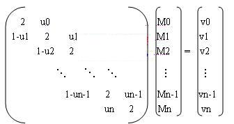
If the boundary condition is assumed to be the natural boundary as described above, then u0 = 0, v0 = 0, un = 0, vn = 0, that is, M0 = Mn = 0.
5 MATLAB to achieve spline interpolation
1.03544329000000 1.03545329000000 1.03546329000000; 0.30182936000000 0.30186004069566 0.30187182180522 0.30186964693605 0.30185845969551 0.30184320369097 0.30182882252981 0.30182025981940 0.30182245916710 0.30184036418029 0.30187889352712 0.30192733665639 0.30193266863021 0.30193987411039 0.30199701768689 0.30198992627645 0.30198730620686 0.30200882997022 0.30203060327638 0.30205012896416 0.30207062461427 0.30209530780615 0.30212717111085 0.30216587747376 0.30220651085041 0.30224372965360 0.30227219229616]